Tutorial
This tutorial introduces basic TensorX concepts.
Prerequisites
TensorX is a machine learning library to build neural network models written in Python and it works as a complement to Tensorflow, therefore, to make the most out of this tutorial (and this library), readers should be familiarized with the following:
- Python 3: if you're new to the Python language or need to refresh some concepts check out the Python Tutorial.
-
Tensorflow: Tensorflow is a high-performance machine learning library that allows numerical computation on GPUs and TPUs. It was originally designed to build auto-differentiable dataflow graphs. Although it has adopted an eager execution model in version 2, computation graphs are still an integral concept of high performance tensorflow program definition and deployment. Unfortunately most tensorflow tutorials and guides, focus on Keras, a high level interface similar to TensorX. For a primer on Tensorflow, I recommend taking a look at Tensorflow basics guide section instead.
-
NumPy: similarly to the core of Tensorflow, Numpy is a numerical computation library with a focus in multi-dimensional array transformations. Given that Tensorflow tensors are converted to and from NumPy arrays, and TensorX also depends on NumPy (mostly for testing), it is recommended that the reader is familiarized with
NumPy basics. For more details, check the NumPy documentation.
Installation
You can install tensorx with pip as follows:
pip install tensorflow
pip install tensorx
for more details see the installation documentation.
Layers
In TensorX, a Layer is the basic building block of a neural network. Semantically speaking, a layer is an object that can have multiple inputs, an inner state, and a computation function applied to its inputs (that depends on the current state). Each layer has a single output. In essence,we can say that a Layer instance is a stateful function. Connecting a series of layers results in a layer graph. In TensorX, each layer is the end-node of a subgraph, and executing it will result in the execution of all layers in the subgraph with the current layer as output. Layer subclasses can range from simple linear transformations (e.g. Layer) to more complex layers used to build recurrent neural networks such as long short-term memory (LSTM) cells (e.g. LSTMCell) or attention mechanisms such as MHAttention.
Layer properties and methods
inputs: list of input layers for the current layer;input: syntax sugar forinputs[0];n_units: number of output units or neurons, this is the last dimension of the output tensor resulting from this layer's computation;shape: the inferred shape for the layer output;compute(*tensors): layer computation applied to its input layers or input tensors if any is given.__call__: all layers are Callable and the result is the computation of the entire layer graph taking the current layer as the terminal node.reuse_with: create a new layer object that shares the state with the current layer but is connected to different inputs. The new layer is the end-point node of a new layer graph.variables: alistoftf.Variableobjects that handled by the current layertrainable_variables: alistoftf.Variableobjects that are trainable, this is, that are changed by an optimizer during training.*config: a layer configuration (LayerConfig) with the arguments used in the current layer instance constructor.
Using existing Layers
TensorX ships with a number of built in Layers that you can easily use to compose layer graphs that perform various
computations. All layers are accessible from the global namespace tensorx.Linear or from the tensorx.layers module.
The following example shows how to use a simple Linear layer that performs the computation
y=Wx+b:
import tensorflow as tf
import tensorx as tx

x = tf.random.uniform([2, 2], dtype=tf.float32)
# y = Wx + b
y = tx.Linear(x, n_units=3)
result = y()

assert tx.tensor_equal(tf.shape(result), [2, 3])
assert len(y.inputs) == 1
assert isinstance(y.input, tx.Constant)
Note that we can pass a Tensor object to Linear (or any other layer), and it will be automatically converted to a
Layer, to a Constant layer to be more precise. The layer y has exactly 1 input layer and __call__ will return
the result of its computation on this input.
Dynamic stateful Input
The Input layer allows us to add a dynamic input to a layer graph:
value = tf.random.uniform([2, 2], dtype=tf.float32)
x = tx.Input(init_value=value)
# y = Wx + b
y = tx.Linear(x, n_units=3)

result1 = y()
# x is stateful and its value can be changed e.g. to a new random value
x.value = tf.random.uniform([2,2], dtype=tf.float32)
result2 = y()
result3 = y.compute(value)

assert not tx.tensor_equal(result1, result2)
assert not y.input.constant
# compute returns the layer computation independently from its current graph
assert tx.tensor_equal(result1, result3)

print(result1)
tf.Tensor(
    [[ 0.8232075   0.2716378  -0.33215973]
     [ 0.34996247 -0.02594224 -0.05033442]],
    shape=(2, 3),
    dtype=float32)
Input allows the creation of dynamic input layers with a value property that
can be changed, we can see that the value at the end-point of this graph changes as well. Moreover,
the compute method is distinct from __call__ as it only depends on the layer current state and
not on the current graph.
Important
if n_units is not set to None on a dynamic Input layer, it will take the last dimension of the initial value,
henceforth, any tensor assigned to value must match the n_units in its last dimension. This means that the batch
dimension can be variable for example.
Warning
You can't switch the number of dimension in a dynamic Input. Without an initial value or shape, it
defaults to a shape (0, 0) (an empty tensor with 2 dimensions). An error is thrown if you try to assign a tensor
with a mismatching number of dimensions. For example, if you create an input as follows
Input(shape=[None,None,None]), an error is thrown if you assign a tensor with a mismatching number of dimensions
like input.value = tf.ones([2,2]).
Re-Using Layers
When you create a new Layer object, usually you will pass it its input layers which will then make it the end-node of
a graph connected to those input layers. This will also call the init_state method which initializes any tf.Variable
objects that might be part of the layers' state. If you want to re-use this layer with a different set of input layers,
you can use the reuse_with method. This creates a new layer with all the same parameters, additionally
this new layer will share it's state with the previous one.
import tensorflow as tf
import tensorx as tx

# stateful input placeholder
x1 = tx.Input(n_units=2)
x1.value = tf.random.uniform([2, 2])
#y = Wx + b
l1 = tx.Linear(x1, n_units=3)
a1 = tx.Activation(l1, tx.relu)
l2 = tx.Linear(a1,n_units=4)

d1 = tx.Dropout(a1,probability=0.4)
l3 = l2.reuse_with(d1)

Warning
Any changes to the state of one layer will affect the state of the second.
Re-Using Modules
A Module is a special layer which creates a single Layer from a given layer graph. A layer graph is a
set of layers connected to each other. For example:
x = tx.Input(tf.ones([2,2]))
y1 = tx.Linear(x,3)
y2 = tx.Linear(y1,4)

m = tx.Module(inputs=x,output=y2)

assert tx.tensor_equal(m(),y2())
You can take the two Linear layers and create a single module with a state shared with both layers. Like with any
other layer you can also call reuse_with on a module and in this case, the entire state of the two Linear layers
will again be shared with the newly created Module.
Gradients and Autodiff
Automatic differentiation is a cornerstone of most deep learning frameworks. TensorFlow remembers what operations
happen and in what order during the forward pass, then, during the backpropagation pass, TensorFlow traverses this list
of operations in reverse order to compute gradients --usually with respect to some input like a tf.Variable.
Automatic differentiation can be accessed in Tensorflow using the tf.GradientTape
context. Whatever is executed inside the GradientTape context, gets tracked so that the gradients with respect to some
variables can be computed:
import tensorflow as tf
x = tf.Variable(3.0)

with tf.GradientTape() as tape:
  y = x**2

# dy = 2x * dx
dy_dx = tape.gradient(y, x)
TensorX Layers describe operations over tensors in terms of tensorflow operations, and store their state in tf.Variable
objects, so layers executed inside the tf.GradientTape context are tracked just like any other Tensorflow operation.
With this in mind, we can then compute the gradients of a particular value with respect to the trainable_variables
used in the computation. For example:
import tensorflow as tf
import tensorx as tx

x = tx.Input(n_units=3)
# y = Wx + b
y = tx.Linear(x, 3, add_bias=True)
loss = tx.Lambda(y, fn=lambda v: tf.reduce_mean(v ** 2))
x.value = [[1., 2., 3.]]

with tf.GradientTape() as tape:
    loss_value = loss()

    # we could have done this as well
    # v = y()
    # loss_value = tf.reduce_mean(v ** 2)

grads = tape.gradient(loss_value, y.trainable_variables)

assert len(y.trainable_variables) == 2
assert len(grads) == 2
assert grads[0].shape == y.weights.shape
assert grads[1].shape == y.bias.shape
In this case, only the weights, and bias of the Linear layer are trainable variables, so we can take the gradient
of loss_value with respect to these variables, the result is a list of tensors with the same shape as the variables
used as targets.
Tip
In these examples we're still using an eager execution model from Tensorflow, as we will see, this is good for
debugging, but not very efficient. Next in this tutorial, we will show how we can compile TensorX layer graphs
into Tensorflow graphs using the tf.function.
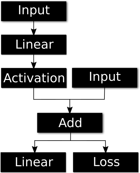
Graph Compilation
TensorX builds layer graphs automatically from layer objects are connected to each other. These graphs are, in effect,
directed acyclic graphs (DAG) defining a given computation over inputs. To aid with validation and execution
of neural network layer graphs, TensorX has a Graph utility class. The Graph class allows for
automatic graph construction from output nodes (by recursively visiting each node's inputs). It also facilitates
transversal by dependency ordering along with conversion of arbitrary graphs to functions and Tensorflow static graphs.
TensorX takes advantage of Tensorflow's graph optimization system to simplify and optimize Layer computations. It does
this by converting layer graphs into functions that are then trace-compiled into an optimized TensorFlow static graphs.
x1 = Input(n_units=2)
x2 = Input(n_units=4)
l1 = Linear(x1,4)
l2 = Add(l1,x2)
l3 = Linear(l2,2)

g = Graph.build(outputs=l3,
                inputs=[x1,x2])
fn = g.as_function(compile=True)
# fn is holding the following function
@tf.function
def compiled_graph():
    x1 = layers["x1"].compute()
    x2 = layers["x2"].compute()
    l1 = layers["l1"].compute(x1)
    l2 = layers["l2"].compute(l1,x2)
    l3 = layers["l3"].compute(l2)
    return l3
If no ord_inputs are given to as_function, the resulting function doesn't define input parameters.
To feed values to such a function we would need to change the values of the inputs with x1.value = ... before
calling fn(). If ord_inputs are passed (e.g. g.as_function(ord_inputs=[x1,x2])), these will map the parameters to the corresponding layers that must
be inputs of the current graph, if so, the resulting function can be called with arguments as fn(value1,value2).
Just as Layer objects define implicit subgraphs, we can also build Callable functions and TensorFlow static graphs
from any layer by calling layer.as_function(). Much like in the previous example, doing this will return a function
without parameters. This is just syntax sugar for:
...
graph = Graph.build(inputs=None, outputs=self)
return graph.as_function(name=name, compile=compile)
Dev Notes
A function conversion procedure which uses parameters with optional values for Input layers is in development.
Models
TensorX uses the Model class to group together multiple layer graphs and simplify the configuration of a training loop with multiple callbacks. This part of the API might suffer some changes but at its core it's just intended as a way to group together layer graphs, optimizers, and a configurable training loop with Callbacks.
Docs in progress
Finish this documentation with examples
Callbacks
Docs in progress
Finish this documentation with examples
Serialization
Docs in progress
Finish this documentation with examples